Impact of Displaying Inpatient Pharmaceutical Costs at the Time of Order Entry: Lessons From a Tertiary Care Center


BACKGROUND: A lack of cost-conscious medication use is a major contributor to excessive healthcare expenditures in the inpatient setting. Expensive medicines are often utilized when there are comparable alternatives available at a lower cost. Increasing prescriber awareness of medication cost at the time of ordering may help promote cost-conscious use of medications in the hospital.
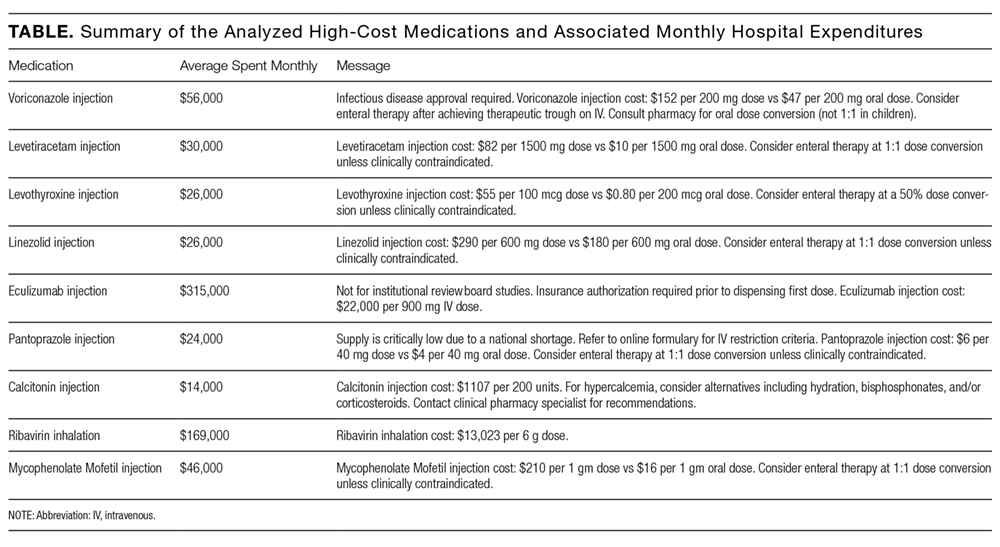
OBJECTIVE: To evaluate the impact of cost messaging on the ordering of 9 expensive medications.
DESIGN: Retrospective analysis of an institutional cost-transparency initiative.
SETTING: A 1145-bed, tertiary care, academic medical center.
PARTICIPANTS: Prescribers who ordered medications through the computerized provider order entry system at the Johns Hopkins Hospital.
METHODS: Interrupted time series and segmented regression models were used to examine prescriber ordering before and after implementation of cost messaging for 9 high-cost medications.
RESULTS: Following the implementation of cost messaging, no significant changes were observed in the number of orders or ordering trends for intravenous (IV) formulations of eculizumab, calcitonin, levetiracetam, linezolid, mycophenolate, ribavirin, and levothyroxine. An immediate and sustained reduction in medication utilization was seen in 2 drugs that underwent a policy change during our study, IV pantoprazole and oral voriconazole. IV pantoprazole became restricted at our facility due to a national shortage (–985 orders per 10,000 patient days; P < 0.001), and oral voriconazole was replaced with an alternative antifungal in oncology order sets (–110 orders per 10,000 patient days; P = 0.001).
CONCLUSIONS: Prescriber cost transparency alone did not significantly influence medication utilization at our institution. Active strategies to reduce ordering resulted in dramatic reductions in ordering. Journal of Hospital Medicine 2017;12: 639-645. © 2017 Society of Hospital Medicine
© 2017 Society of Hospital Medicine
Variables
“Week” and “month” were defined as the week and month of our study, respectively. The “period identifier” was a binary variable that identified the time period before and after the intervention. “Weekly orders” was defined as the total number of new orders placed per week for each specified drug included in our study. For example, if a patient received 2 discrete, new orders for a medication in a given week, 2 orders would be counted toward the “weekly orders” variable. “Patient days,” defined as the total number of patients treated at our facility, was summated for each week of our study to yield “weekly patient days.” To derive the “number of weekly orders per 10,000 patient days,” we divided weekly orders by weekly patient days and multiplied the resultant figure by 10,000.
Statistical Analysis

Segmented regression, a form of interrupted time series analysis, is a quasi-experimental design that was used to determine the immediate and sustained effects of the drug cost messages on the rate of medication ordering.15-17 The model enabled the use of comparison groups (alternative medications, as described above) to enhance internal validity.
In time series data, outcomes may not be independent over time. Autocorrelation of the error terms can arise when outcomes are more similar at time points closer together than outcomes at time points further apart. Failure to account for autocorrelation of the error terms may lead to underestimated standard errors. The presence of autocorrelation, assessed by calculating the Durbin-Watson statistic, was significant among our data. To adjust for this, we employed a Prais-Winsten estimation to adjust the error term (εt) calculated in our models.
Two segmented linear regression models were used to estimate trends in ordering before and after the intervention. The presence or absence of a comparator drug determined which model was to be used. When only single medications were under study, as in the case of eculizumab and calcitonin, our regression model was as follows:
Yt = (β0) + (β1)(Timet) + (β2)(Interventiont) + (β3)(Post-Intervention Timet) + (εt)
In our single-drug model, Yt denoted the number of orders per 10,000 patient days at week “t”; Timet was a continuous variable that indicated the number of weeks prior to or after the study intervention (April 10, 2015) and ranged from –116 to 27 weeks. Post-Intervention Timet was a continuous variable that denoted the number of weeks since the start of the intervention and is coded as zero for all time periods prior to the intervention. β0 was the estimated baseline number of orders per 10,000 patient days at the beginning of the study. β1 is the trend of orders per 10,000 patient days per week during the preintervention period; β2 represents an estimate of the change in the number of orders per 10,000 patient days immediately after the intervention; β3 denotes the difference between preintervention and postintervention slopes; and εt is the “error term,” which represents autocorrelation and random variability of the data.
As mentioned previously, alternative dosage forms of 7 medications included in our study were utilized as comparison groups. In these instances (when multiple drugs were included in our analyses), the following regression model was applied:
Y t = ( β 0 ) + ( β 1 )(Time t ) + ( β 2 )(Intervention t ) + ( β 3 )(Post-Intervention Time t ) + ( β 4 )(Cohort) + ( β 5 )(Cohort)(Time t ) + ( β 6 )(Cohort)(Intervention t ) + ( β 7 )(Cohort)(Post-Intervention Time t ) + ( ε t )