Chi-square and Fisher’s exact tests


Returning to the lung morphology and mortality example, were the assumptions met? The data consist of 105 unique patients. Thus, we can assume that they are independent. The minimum expected count was 10.9, which is not less than 5. Therefore, the assumptions for the chi-square test are met. Next, the test statistic is calculated using the observed and expected counts. For each cell, subtract the expected count from the observed count, square it, and divide by the expected count. Then, add the 4 resulting numbers to obtain the test statistic of 4.92.
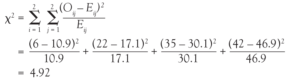

Finally, compute the area under the chi-square distribution with 1 degree of freedom Χ2(1), at the test statistic and values more extreme. In this case, values more extreme are values greater than the test statistic. Here, the area under the curve to the right of 4.92 is .027 (Figure 3). This is the P value, which indicates that the data and the null hypothesis have very low compatibility. In this example, the area under the curve to the right of 4.92 is .027 (Figure 3). This is the P value, which indicates that the data and the null hypothesis have very low compatibility. Thus, the decision is to reject the null hypothesis. The conclusion is that lung morphology is associated with 90-day mortality (P = .027). To describe that association, one looks at the contingency table and finds a reduction in 90-day mortality with focal patterns compared to nonfocal patterns (21.4% vs 45.5%, respectively). The P value reported in the article is .026. Our hand calculation was .027, which is slightly off due to rounding. In summary, the scenario is an investigation into the association among 2 categorical variables, and, thus, a test to consider is the chi-square test, if assumptions are met.
In another example in the same study, the authors investigate whether any baseline characteristics are associated with lung morphology. For example, is neurology, specifically Parkinson disease (yes vs no), associated with lung morphology (focal vs nonfocal)? Again, the scenario is an investigation into the association between 2 categorical variables, so a chi-square test should be considered.

To start, build a contingency table arbitrarily placing lung morphology as the row variable and Parkinson disease as the column variable. Populate the contingency table based on the counts and percentages reported in the article (Figure 4). Next, check that the assumptions of the chi-square test are met. Are the observations independent? Again, because these are unique patients, we consider this assumption met. Since this is a 2 × 2 table, are all of the expected counts greater than 5? Calculations of the expected counts obtained the following: 1.1, 30.9, 2.9 and 84.1. Here, 2 of the 4 expected counts are less than 5. Therefore, methods that use large sample approximation, like the chi-squared test, may not be an appropriate choice.
Instead of using methodology that is an approximation, consider an exact test such as Fisher’s exact test. Again, refer to the contingency table where Fisher’s exact is going to calculate the exact probability (under the null hypothesis) of the observed data or results more extreme. This is the technical definition of a P value. It is, however, still quantifying how compatible the data are with the null hypothesis. The exact probability of a particular contingency table can be obtained using the hypergeometric distribution.
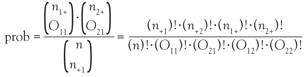
The symbols that resemble large parentheses are notations for a combinatorial. Because using combinatorials to calculate the probability is not user friendly, an equivalent version relies on factorials instead. Both techniques are presented above. Remember that the goal is to find the exact probability of the observed data or something more extreme.
The hypotheses are still testing whether these 2 categorical variables are associated with each other. In this particular example, we test if the proportion of patients with Parkinson disease is the same in the focal and nonfocal groups. Fisher’s exact test obtains its two-tailed P value by computing the probabilities associated with all possible tables that have the same row and column totals. Then, it identifies the alternative tables with a probability that is less than that of the observed table. Finally, it adds the probability of the observed table with the sum of the probabilities of each alternative table identified above, which results in the P value.

To explore each of those steps in detail, one must first enumerate how many tables can be built that all have the same row and column totals as the observed table. Figure 5 shows the 5 possible tables. Pick any one of the 5 2 × 2 tables; the margins are fixed. Each table has the same row totals, 32 focal and 87 nonfocal, and each table has the same column totals: 4 Parkinson and 115 non-Parkinson. Then, for each table, calculate the probability of that table. Figure 5 shows this calculation for the first 2 × 2 table, which happens to be the observed table. The probability of the table observed in the study is .2803. Such a calculation is performed on each of the other tables.
Next, one must identify the tables that have a probability smaller than the observed table. Here, we are looking for probabilities less than .2803. These are the tables deemed more extreme. Tables 3, 4, and 5 have probabilities less than .2803.