Chi-square and Fisher’s exact tests

Once the contingency table is built, the question becomes, “Is lung morphology associated with 90-day mortality?” To answer that question, we need to know how many patients one would expect in each table cell if the null hypothesis of no association is true. When conducting a hypothesis test, one always assumes that the null hypothesis is true and then gathers data to see how well the data aligns with that assumption.

So one must calculate how many patients to expect in each of these cells if lung morphology is not associated with 90-day mortality. One way to address this question is to ask these 2 questions:

(1) Overall, what proportion of patients die by day 90? Looking at the constructed contingency table, that answer would be 39%. This was calculated by taking the total number of patients who died by day 90 and dividing it by the total number of patients, 41/105 = 39%. This gives the overall proportion, based on the data, who would die by day 90.

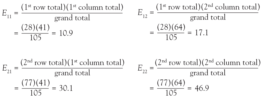
(2) How many of the focal ARDS patients would be expected to die by day 90? Now it is not overall, but rather we are limiting the question to the focal ARDS group. To obtain the answer, multiply the overall proportion of patients who die by day 90 by how many focal ARDS patients are in the study. Essentially, take the answer from the previous question and multiply it by the total number of focal ARDS, which is 28. The result is (41/105) × 28 = 10.9. Thus, if there is no association among long morphology and 90-day mortality, one would expect 10.9 focal ARDS patients to die by day 90.

Now 10.9 is a very specific answer for a specific contingency table, but the answer could be written in general terms. Basically, 3 numbers were used in calculating the solution: the row margin, the column margin, and the grand total. The general formula is the following:

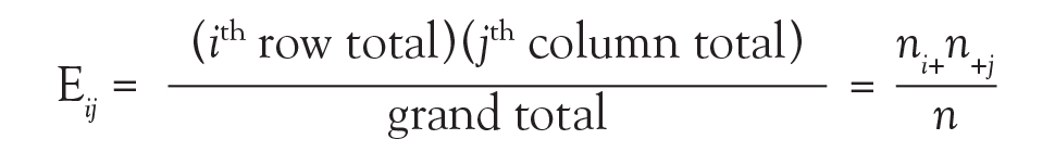
The notation E_ij is used to represent the expected count assuming the null hypothesis of no association among the row and column variables is true. To calculate the expected count, take the i^th row total times the j^th column total and divide by the grand total.

In the lung morphology and mortality example, what is the expected number of deaths within 90 days among the nonfocal ARDS patients? This is the second row and the first column (E₂₁). Applying the formula, one multiplies the total for the second row by the total for the first column and then divides by the grand total, (77 × 41)/105 = 30.1. This calculation is repeated for each of the 4 cells.

Because we now know the observed cell count and the expected cell count (under the null hypothesis), we can compare the observed and expected counts to see how well the data aligns with the null hypothesis. This is what the chi-square test does, and the test statistic is calculated as follows:

The sigma (Σ) means addition, so the calculation is performed on each individual cell in the contingency table and then the results are summed. A 2 × 2 table has 4 cells and thus 4 numbers will be summed. For each cell, the formula compares the observed to the expected. Basically, it computes how similar they are (that is the O minus E part). Because the differences will be positive for some cells and negative for others, the differences are squared to avoid cancellation when you add them. Finally, each squared difference is divided by the expected count to standardize the calculation.

Intuitively, if the observed counts (O_ij) are similar to the expected counts under the null hypothesis (E_ij), then these 2 numbers will be very close to each other. When taking the difference between them or subtracting them, the result is a small number. When squaring a small number, one obtains a really small number. And adding up a bunch of really small numbers results in a small number. So the test statistic is going to be small. That means that the resulting P value is going to be large. What is a P value? Think of it as an index of compatibility. How compatible is the data with the null hypothesis? Here, you get a large index of compatibility. That means that the data aligns nicely with the null hypothesis and one fails to reject the null.

Now, think about the alternative scenario. If the observed counts (O_ij) are wildly different from the expected counts under the null hypothesis (E_ij), then these 2 numbers will be quite different. When taking the difference between them or subtracting them, the result is a big number. When squaring a big number, one obtains a really big number, and adding up a bunch of really big numbers results in a large number. So the test statistic is going to be large. That means that the resulting P value is going to be small. And if you think of a P value as an index of compatibility, the data and the null hypothesis are not very compatible. That means that the data does not align nicely with the null hypothesis and one rejects the null. This is the general idea of the chi-square test. It assesses how compatible the data is with the null hypothesis that the 2 categorical variables are not associated.

To obtain the actual P value, the distribution of the test statistic (under the null hypothesis) is used to calculate the area under the curve for values equal to the test statistic or more extreme. The described test statistic has an approximate chi-square distribution with (r − 1)(c − 1) degree of freedom. Recall that r is the number of levels of the row variable and c is the number of levels of the column variable. Our example is a 2 × 2 table, so the test statistic has an approximate chi-square distribution with (2 − 1)(2 − 1) = 1 degree of freedom.

Now that the chi-square test has been fully described, the assumptions for the test must be discussed. It is important to know when you should or should not perform this test. The chi-square test assumes that observations are independent. This means that the outcome for one observation is not associated with the outcome of any other observation. This principle can be violated when multiple measurements are taken over time or when multiple measurements are taken from one patient.

Another assumption is that the chi-square large sample approximation just described is appropriate. In other words, no more than 20% of the expected counts (E_ij) are less than 5. For a 2 × 2 table, how many cells do you have? Four. So if even one of those 4 happens to have an expected count less than 5, this assumption is violated. For a 2 × 2 table, none of the expected counts can be less than 5.